Backtesting a Mean-Reverting Trading Strategy using the Johansen test

Backtesting a mean-reversion strategy using the Johansen test. Python code included.

Oct 22, 2023

In last week’s article, we walked through how to create a stationary time series from two non-stationary time series using the Engle-Granger test. If you haven’t read it yet, check it out here.

The biggest drawback of this method is that it can only be applied to two time series.

The Johansen test enables us to construct a stationary time series using three or more non-stationary time series. Thus the Johansen test can be applied to a larger variety of time series data.

In this article you will:

Learn about the Johansen test
Construct a stationary portfolio using the Johansen test
Backtest a mean-reverting strategy based on the Johansen test

Johansen Test

First, the data is fit to a Vector Error Correction Model (VECM) which is shown below.

The Johansen test is conducted by performing an eigenvalue decomposition of A. The rank of the matrix A is given by r and the Johansen test sequentially tests whether the rank r=0, r=1, …., r=n−1, where n is the number of time series under test.

The null hypothesis of r=0 means that there is no cointegration at all. A rank r>0 implies a cointegrating relationship between two or possibly more time series.

The eigenvector corresponding to the largest eigenvalue contains the coefficients of the linear combination which shall be used to transform the original non-stationary time series into a stationary portfolio time series.

If you’d like to learn about the mathematics behind the Johansen test in more detail check out this article.

Imports

%%capture
!pip install yfinance

import numpy as np
import pandas as pd
import yfinance as yf
import matplotlib.pyplot as plt
from statsmodels.tsa.vector_ar.vecm import coint_johansen

Initialise Parameters

stock_tickers = [
    'AAPL', 'GOOGL', 'MSFT', 'NVDA', 'INTC', # Technology Sector
    'JNJ', 'PFE', 'UNH', 'ABBV', 'GILD', # Healthcare Sector
    'XOM', 'CVX', 'COP', 'OXY', 'SLB', # Energy Sector
    'PG', 'KO', 'PEP', 'NKE', 'K', # Consumer Goods Sector
    'JPM', 'BAC', 'C', 'GS', 'AXP', # Financial Sector
]

train_start = '2021-01-01'
train_end = '2023-01-31'

Download Stock Data

stock_data = yf.download(stock_tickers, 
                         start=train_start, 
                         end=train_end)['Adj Close']
stock_data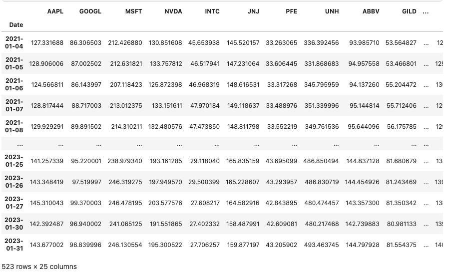

Johansen Test Implementation

data_arr = np.array(stock_data)

result = coint_johansen(data_arr, det_order=0, k_ar_diff=1)

eigenvalues = result.eig
eigenvectors = result.evec
eig_statistic = result.max_eig_stat
eig_critical_values = result.max_eig_stat_crit_vals

Construct a Stationary Portfolio

coint_vector = eigenvectors[:, 0]

portfolio = np.dot(data_arr, coint_vector)

portfolio_df = pd.DataFrame(portfolio, columns=['portfolio'])

portfolio_df.plot()

Backtest

The mean reversion trading signal is based on a simple z-score strategy, as described in my previous article.

portfolio_df['returns'] = np.log(portfolio_df['portfolio'] / portfolio_df['portfolio'].shift(1))

portfolio_df['mean'] = portfolio_df['portfolio'].mean()

portfolio_df['std'] = portfolio_df['portfolio'].std()

portfolio_df['position'] = -(portfolio_df['portfolio'] - portfolio_df['mean']) / portfolio_df['std']

portfolio_df['daily returns'] = portfolio_df['returns'] * portfolio_df['position'].shift(1)

portfolio_df['cum returns'] = portfolio_df['daily returns'].cumsum()

Plot PnL

plt.figure()
portfolio_df['cum returns'].plot()
plt.title('Johansen Test Mean Reversion Strategy PnL')
plt.xlabel('Time')
plt.ylabel('PnL')
plt.grid()